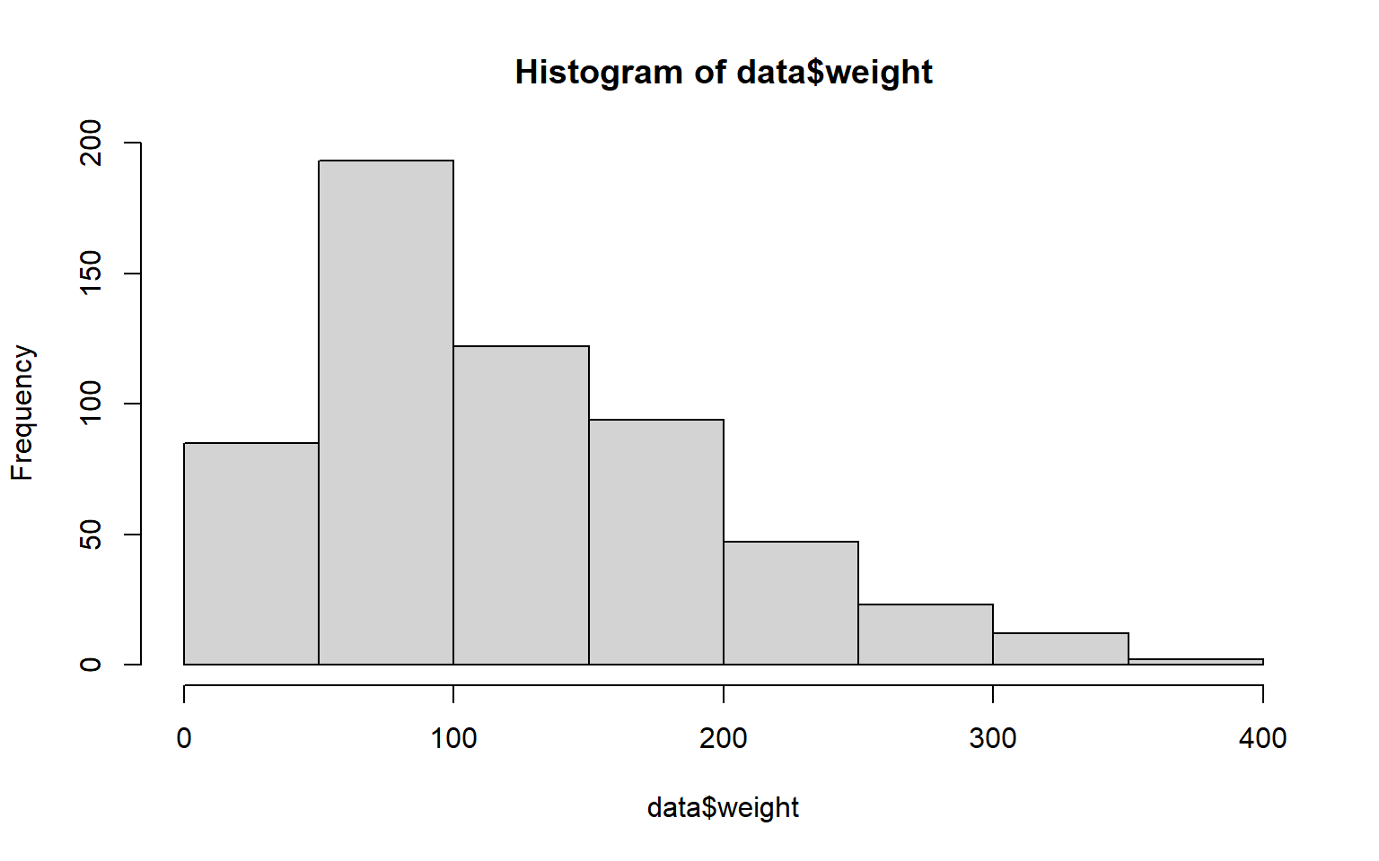
The hist() function can be used to make a simple histogram. Here, we are graphing weights of chicks from the built-in R dataset “ChickWeight”
data(ChickWeight)
data <- ChickWeight
hist(data$weight)
Output:
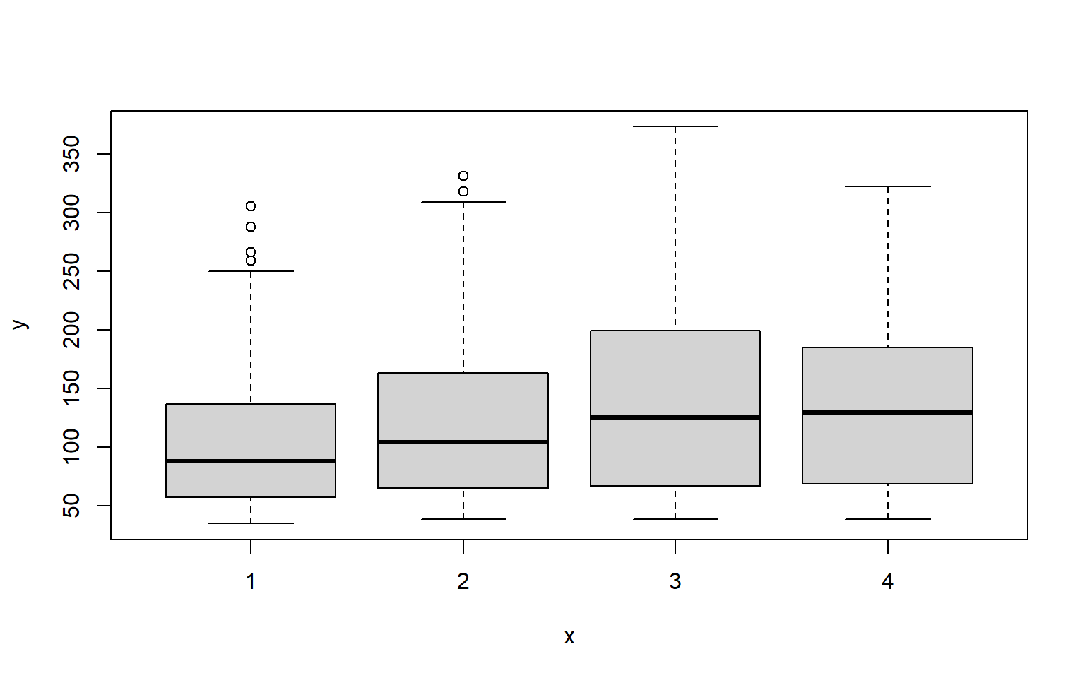
We can also use the plot() command for some simple graphing. Here, we will plot chick weight as a function of chick diet. Because Diet is categorical, the plot() command will automatically plot our data as a set of box and whisker plots.
plot(y=data$weight, x=data$Diet)
Output:
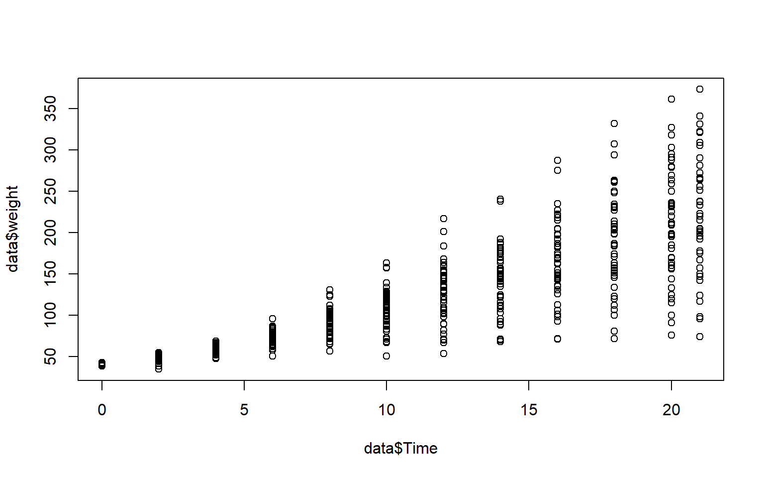
If we use a non-categorical variable like Time, we can see that the plot() command changes how it displays the data. Here, it is plotting raw data points.
plot(y=data$weight, x=data$Time)
Output:
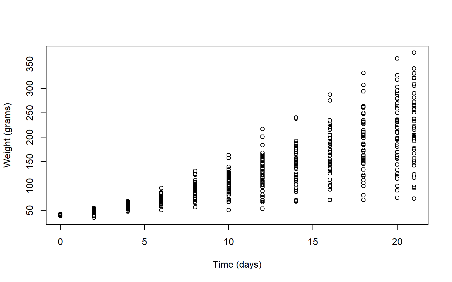
With the plot() command, we can also add x and y axis labels with “xlab = " and “ylab = “.
plot(y=data$weight, x=data$Time, xlab="Time (days)", ylab="Weight (grams)")
Output:
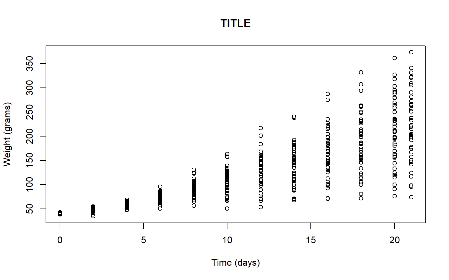
And, we can add a title using “main = "
plot(y=data$weight, x=data$Time, xlab="Time (days)", ylab="Weight (grams)", main='TITLE')
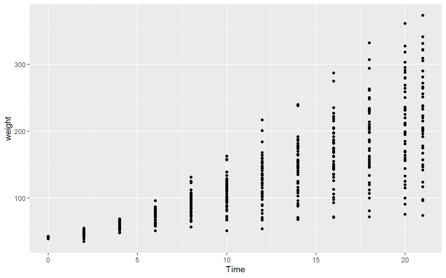
For more control over our figures, we can use the ggplot() function from the ggplot2 library. This function works by adding different ggplot objects together, to make a full figure. Here, we will start by setting Time to the x axis, Weight to the y axis, and adding a “geom_point” object – this will plot data as points.
library(ggplot2)
ggplot(data, aes(x = Time, y = weight))+  geom_point()
Output:
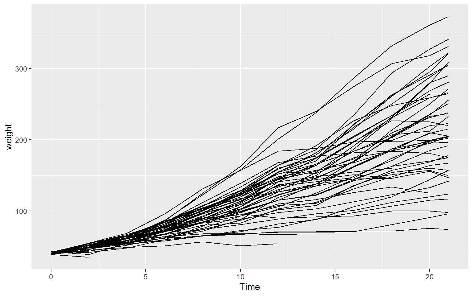
We can graph our data with lines as well. This will require adding a geom_line object, and telling ggplot what variable we want our data to be grouped by (in this case, our data will be grouped by individual Chick identities).
ggplot(data, aes(x = Time, y = weight, group = Chick))+ geom_line()
Output:
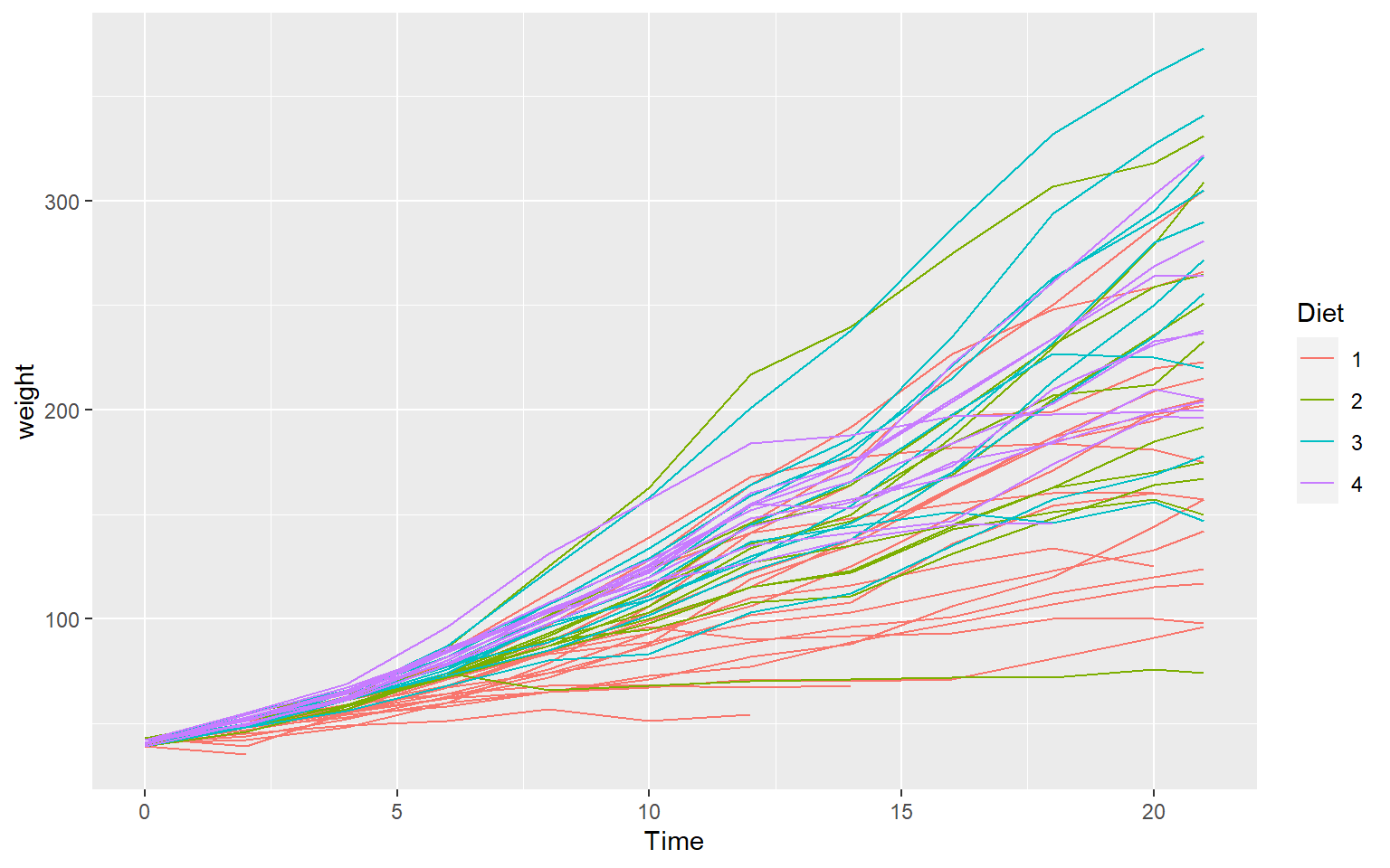
We can set our lines to be different colors depending on which category of a variable they are in. Here, we will color our lines differently by different chick Diets.
ggplot(data, aes(x = Time, y = weight, color = Diet, group = Chick))+ geom_line()
Output:
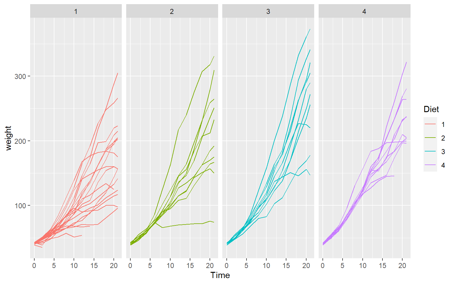
To make data like this look a little less crazy, we can also facet our graph into smaller sub-graphs. We can do this with facet_grid(. ~Variablename). This means that, each category of that chosen variable (here we are using Diet again) will be displayed in a different subsection.
ggplot(data, aes(x = Time, y = weight, color = Diet, group = Chick))+ geom_line()+ facet_grid(. ~ Diet)